Lecture notes and code samples from ML Foundations Summer School in Bilimler Koyu. The notebook is based largely on the following resources:
The text is generated by ChatGPT - after careful prompting 😋
Import statements
import torch
import torch.nn as nn
import torch.nn.functional as F
from torch.utils.data import Dataset, DataLoader
from torch.nn.utils.rnn import pad_sequence

from torchvision.datasets import CIFAR10
from torchvision import transforms

import numpy as np
import matplotlib.pyplot as plt

from datasets import load_dataset
from transformers import AutoTokenizer

device = torch.device('cuda' if torch.cuda.is_available() else 'cpu')
/mnt/lustre/work/vernade/cyildiz40/.conda/sumsch/lib/python3.11/site-packages/tqdm/auto.py:21: TqdmWarning: IProgress not found. Please update jupyter and ipywidgets. See https://ipywidgets.readthedocs.io/en/stable/user_install.html
  from .autonotebook import tqdm as notebook_tqdm
The main task in this notebook
We will learn a higher-order Markovian model that
- takes as input some context that has length more than 1
- predicts the future based on the context: \begin{align*} p(x_0, x_1, \ldots, x_N) = p(x_0) \prod_{n=1}^N p(x_n | x_{<n}) \end{align*}
This model will translate German to English. Let's see what the dataset looks like.
tok = AutoTokenizer.from_pretrained("Helsinki-NLP/opus-mt-de-en")

if tok.bos_token is None:
    tok.add_special_tokens({"bos_token": "<bos>"})
if tok.pad_token is None:
    tok.add_special_tokens({"pad_token": "<pad>"})
if tok.eos_token is None:
    tok.add_special_tokens({"eos_token": "<eos>"})

print('Vocab size:', len(tok))

ds_train = load_dataset("bentrevett/multi30k", split="train")   # fields: "de", "en"
ds_valid = load_dataset("bentrevett/multi30k", split="validation")

# Peek at the first example
print(len(ds_train), 'data points.')
print('\nAn example data point:', ds_train[0])

de_en = '[DE] ' + ds_train[0]['de'] + ' [EN] ' + ds_train[0]['en']
print('\nInput-outputs derived from the first data point:')

split_de_en = de_en.split(' ')
for i in range(14,23):
    print('\nInput:', ' '.join(split_de_en[:i]))
    print('Output:', ' '.join(split_de_en[i:i+1]))


# print('\nInput:', de_en[:76])
# print('Output:', de_en[76:79])

# print('\nInput:', de_en[:80])
# print('Output:', de_en[80:85])

# print('\nInput:', de_en[:87])
# print('Output:', de_en[87:92])

# print('\nInput:', de_en[:93])
/mnt/lustre/work/vernade/cyildiz40/.conda/sumsch/lib/python3.11/site-packages/transformers/models/marian/tokenization_marian.py:175: UserWarning: Recommended: pip install sacremoses.
  warnings.warn("Recommended: pip install sacremoses.")
Vocab size: 58102
29000 data points.

An example data point: {'en': 'Two young, White males are outside near many bushes.', 'de': 'Zwei junge weiße Männer sind im Freien in der Nähe vieler Büsche.'}

Input-outputs derived from the first data point:

Input: [DE] Zwei junge weiße Männer sind im Freien in der Nähe vieler Büsche. [EN]
Output: Two

Input: [DE] Zwei junge weiße Männer sind im Freien in der Nähe vieler Büsche. [EN] Two
Output: young,

Input: [DE] Zwei junge weiße Männer sind im Freien in der Nähe vieler Büsche. [EN] Two young,
Output: White

Input: [DE] Zwei junge weiße Männer sind im Freien in der Nähe vieler Büsche. [EN] Two young, White
Output: males

Input: [DE] Zwei junge weiße Männer sind im Freien in der Nähe vieler Büsche. [EN] Two young, White males
Output: are

Input: [DE] Zwei junge weiße Männer sind im Freien in der Nähe vieler Büsche. [EN] Two young, White males are
Output: outside

Input: [DE] Zwei junge weiße Männer sind im Freien in der Nähe vieler Büsche. [EN] Two young, White males are outside
Output: near

Input: [DE] Zwei junge weiße Männer sind im Freien in der Nähe vieler Büsche. [EN] Two young, White males are outside near
Output: many

Input: [DE] Zwei junge weiße Männer sind im Freien in der Nähe vieler Büsche. [EN] Two young, White males are outside near many
Output: bushes.
1. Introduction
Different architectures
Over the past decades, machine learning has produced many different architectures, each suited to different kinds of data:
- Multilayer perceptrons (MLPs) were the earliest general-purpose neural networks, used for tasks like basic classification and regression.
- Convolutional neural networks (CNNs) then became the workhorse for computer vision, learning how to recognize patterns in images by exploiting local structure.
- For sequential data, recurrent neural networks (RNNs) were widely adopted, because they could process variable-length sequences by maintaining a hidden state over time. A prominent example of RNNs in practice was machine translation, where models such as the Sequence-to-Sequence architecture (Sutskever et al., 2014, figure below) with attention mechanisms (Bahdanau et al., 2015) achieved major breakthroughs.
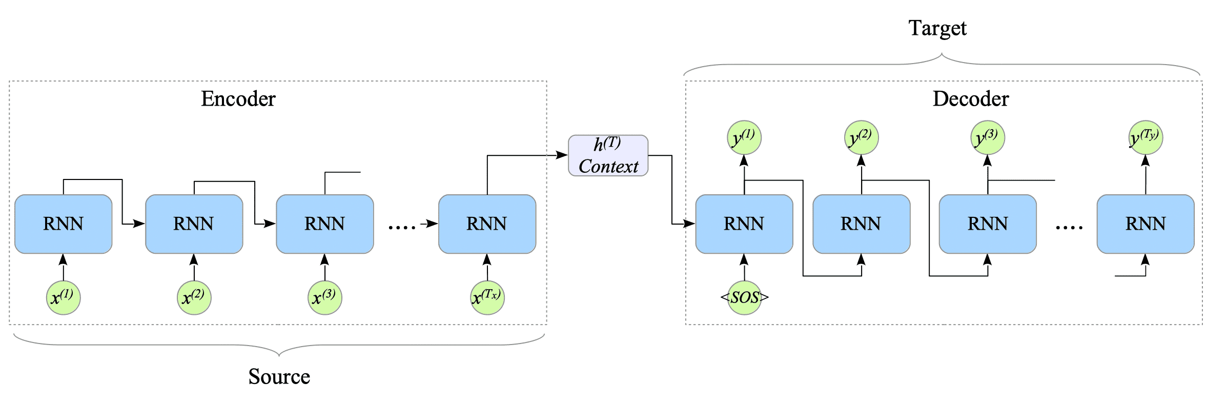
A cartoon illustration of RNN-based machine translation (image from https://www.interdb.jp/dl/part03/ch13.html)
Attention
The idea of attention itself was revolutionary. It allowed models to dynamically focus on the most relevant parts of the input, instead of compressing everything into a single fixed-size vector. Early applications included neural machine translation, image captioning, and speech recognition. But then came a turning point: the landmark paper “Attention Is All You Need” (Vaswani et al., 2017). This work proposed the Transformer, a model built entirely around attention layers, without recurrence or convolutions. It introduced the now-famous encoder–decoder architecture, where the encoder transforms an input sequence (like a German sentence) into a sequence of contextual representations, and the decoder generates the output sequence (like the English translation) step by step, attending both to the encoder’s outputs and to its own past predictions.
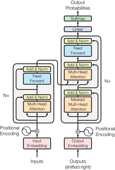
Attention is all you need architecture (image from Vaswani et al., 2017)
Causal language models
The Transformer quickly became the dominant architecture for language tasks, and soon spread to vision, speech, and beyond. But in this tutorial, our focus will not be on faithfully reproducing the exact “Attention Is All You Need” setup. Instead, we’ll study the core building blocks — attention, masking, autoregression — through the lens of causal language models (LLMs). These models, like GPT-2 (Radford et al., 2019) and its descendants, use the Transformer in a simpler “decoder-only” form, where the goal is always the same: predict the next token given the previous ones. By starting here, we’ll build a clear intuition for how modern translation and large-scale language models are trained.
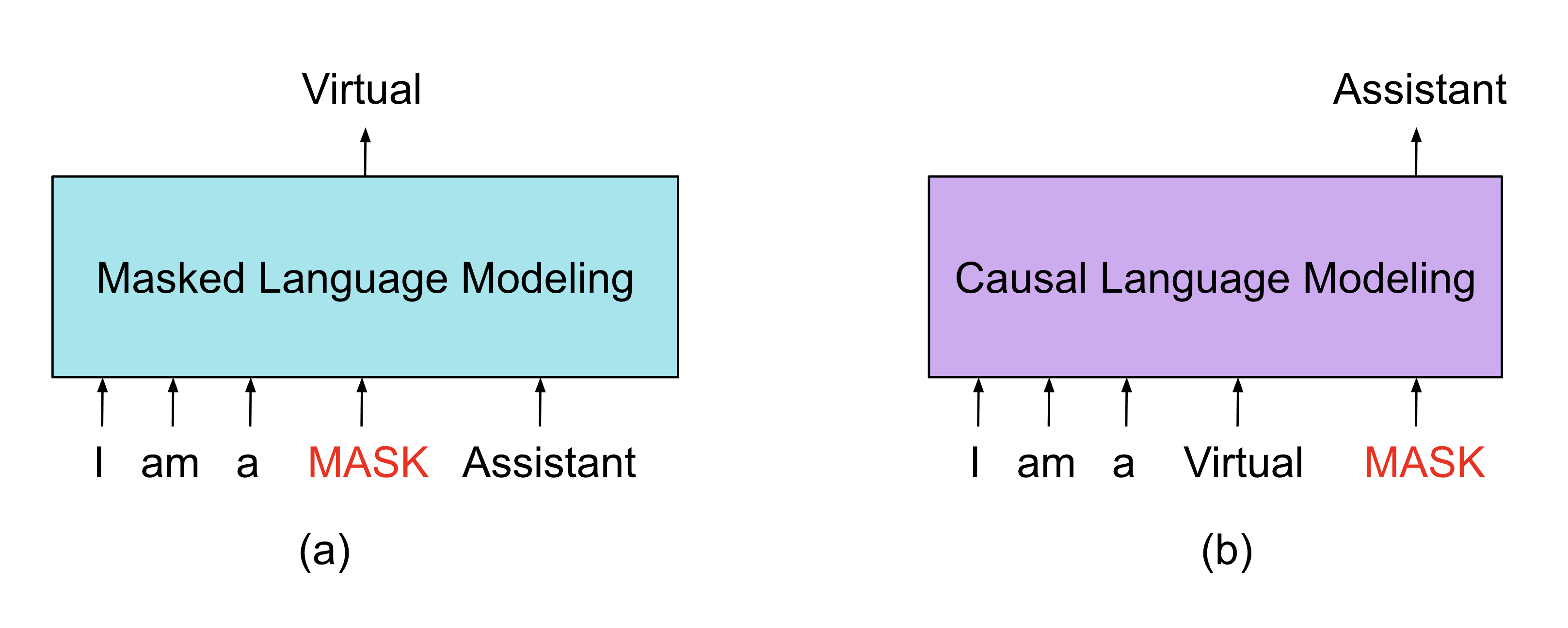
Causal vs masked language models (image from https://www.holisticai.com/blog/from-transformer-architecture-to-prompt-engineering)
What are we going to implement?
1. A Transformer network
We will implement, from scratch, a transformer network. This network will be quite generic - so much so that it could be used even for computer vision as we demonstrate at the end of this notebook.
2. Auto-regressive (causal) next item predictors
A central idea in sequence modeling is auto-regression: given a sequence of items, a model learns to predict the next item based on the context of all previous ones. Here, the model could be any ML model, and we will consider MLPs and Transformers. This approach is powerful because it transforms the problem of modeling complex sequences into a series of simple, repeated predictions. For text, this means predicting the next word given the words that came before; for time series, it could mean predicting tomorrow’s value from past values. Once trained, such a model can be used to generate arbitrarily long sequences: start with an initial context, predict the next token, append it to the context, and repeat. This is the principle behind modern large language models like GPT.
3. Data loaders and training modules
Of course, we would like to see if our method actually works or not. For this, we will consider a German-to-English translation dataset
T = 256     # Context length (sequence length)
V = 10000   # Vocabulary size (for embeddings)
N = 12      # Number of Transformer blocks
d = 256     # Embedding dimension
H = 8       # Number of attention heads

class TransformerNetwork(nn.Module):
    def __init__(self, T, N, input_emb, pos_emb, transf_block, norm_layer, output_layer):
        ''' Transformer network with N blocks, context length T, and given components.
        Args:
            T: Context length (sequence length).
            N: Number of Transformer blocks.
            input_emb: Input embedding layer/module.
            pos_emb: Positional embedding layer/module.
            transf_block: A single Transformer block (to be repeated N times).
            norm_layer: Normalization layer/module (e.g., LayerNorm).
            output_layer: Output layer/module (e.g., for classification or regression).
        '''
        super(TransformerNetwork, self).__init__()
        self.T = T
        self.input_emb = input_emb
        self.pos_emb = pos_emb
        self.transf_blocks = nn.ModuleList([transf_block for _ in range(N)])
        self.norm_layer = norm_layer
        self.output_layer = output_layer

    @property
    def device(self):
        return next(self.parameters()).device

    @property
    def dtype(self):
        return next(self.parameters()).dtype

    @property
    def num_layers(self):
        return len(self.transf_blocks)

    @property
    def d(self):
        return self.input_emb.embedding_dim

    def forward(self, X):
        '''
        Forward pass through the Transformer network.
        Args:
            X: Input tensor of shape (batch_size, T, input_dim), or (B,T,d).
        Returns:
            Output tensor after passing through the Transformer network.
        '''
        device = X.device
        B,T = X.shape[0:2]
        # assert T == self.T, f'Input sequence length {T} does not match model context length {self.T}.'

        # Input embedding
        X  = self.input_emb(X)  # B,T,d

        # positional embeddings
        P  = self.pos_emb(torch.arange(T, device=device)) # T,d
        P  = P.unsqueeze(0).expand(B, T, -1)  # B,T,d

        # adding positional embeddings
        X = X + P  # B,T,d

        # passing through Transformer blocks
        for block in self.transf_blocks:
            X = block(X)  # B,T,d

        # final normalization
        X = self.norm_layer(X)  # B,T,d

        # output layer
        out = self.output_layer(X)  # B,T,output_dim (depends on output_layer)

        return out
2.2. Embeddings and positional encodings
At the input layer, tokens are first mapped into embeddings, and we add positional encodings so the model can take the token order into account. The sequence of embeddings is then passed through a stack of Transformer blocks:
- Embeddings: Neural networks cannot work directly with discrete symbols (like words or image patches), so we map them into continuous vectors called embeddings. These vectors capture semantic or structural properties in a way that the model can process. In NLP, embeddings represent tokens such that similar words are close in vector space; in vision, embeddings represent image patches or regions in a comparable way.
- Positional encodings: Transformers do not have an inherent sense of order, since self-attention treats all tokens symmetrically. To provide the model with information about sequence or spatial position, we add positional encodings to the embeddings. In text, this means encoding word positions within a sentence; in vision, it means encoding the 2D location of a patch within an image. These positional signals let the model distinguish, for example, “the first word in a sentence” or “a patch in the top-left corner of an image.”
def create_embedding(input_dim, output_dim):
    ''' Creates an embedding layer for input tokens. '''
    return nn.Embedding(input_dim, output_dim)

input_emb = create_embedding(V, d) # Input embedding
pos_emb   = create_embedding(T, d) # Positional embedding

# example usage of positiona embeddings
P = pos_emb(torch.arange(T)) # Example usage to get positional embeddings for positions 0 to T-1
plt.figure(figsize=(8,4))
plt.imshow(P.detach().cpu().numpy(), aspect='auto')
plt.colorbar()
plt.title('Positional Embeddings (not trained yet)')
plt.xlabel('Embedding Dimension')
plt.ylabel('Position')
plt.show()

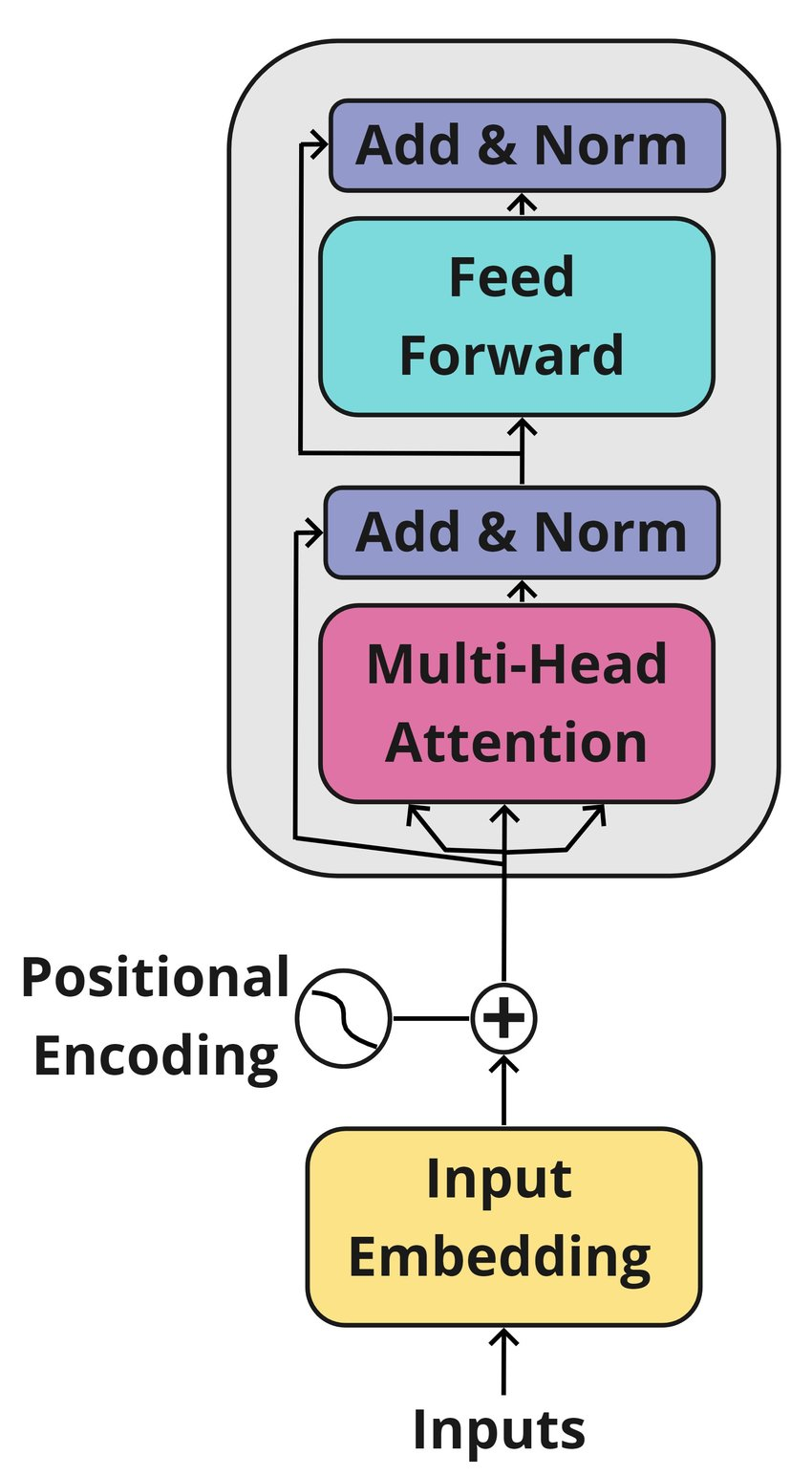
2.3. Transformer blocks
Each Transformer block has two main components:
- Multi-Head Self-Attention (MHSA), which allows every token to attend to other tokens in the sequence, gathering relevant context.
- Feed-Forward Network (FFN), a small MLP applied to each token representation independently.
Both parts are wrapped with residual connections and layer normalization for stable training.
- Layer normalization works by normalizing the activations of each token representation across its hidden dimensions, ensuring that values have consistent scale and distribution. This helps gradients flow more reliably, reduces sensitivity to initialization, and allows the model to train deeper networks without diverging. In practice, it is usually applied together with residual connections, so that the model learns new information while preserving the original signal.
class Block(nn.Module):
    def __init__(self, mhsa, d, d_ff, dropout=0.1):
        ''' A single Transformer block with Multi-Head Self-Attention and Feed-Forward Network.
        Args:
            mhsa: Multi-Head Self-Attention module.
            d: Embedding dimension.
            d_ff: Dimension of the feed-forward network.
            dropout: Dropout rate.
        '''
        super(Block, self).__init__()
        self.mhsa = mhsa
        self.ffn  = nn.Sequential(
            nn.Linear(d, d_ff),
            nn.ReLU(),
            nn.Linear(d_ff, d)
        )
        self.norm1 = nn.LayerNorm(d)
        self.norm2 = nn.LayerNorm(d)
        self.dropout = nn.Dropout(dropout)

    def forward(self, X):
        '''
        Forward pass through the Transformer block.
        Args:
            X: Input tensor of shape (B, T, d).
        Returns:
            Output tensor of shape (B, T, d).
        '''
        X = X + self.dropout(self.mhsa(self.norm1(X)))
        X = X + self.dropout(self.ffn(self.norm2(X)))
        return X
2.4. Self-attention implementation
Within attention, the terms query, key, and value have special meaning:
- A query vector represents the current token asking “what information do I need?”
- Key vectors represent all tokens as potential “addresses” to look up.
- Value vectors hold the actual information to be passed along.
Attention works by comparing queries against keys (using dot products), producing weights that determine how strongly each token’s value contributes to the output. This mechanism lets the model learn what to pay attention to at every step.
For an input $X = x_{1:n}$, where each token $x \in \mathbb{R}^d$, we first obtain queries, keys and values:
\begin{align} Q &= W_q^\top X \in \mathbb{R}^{n\times d_q}\\ K &= W_k^\top X \in \mathbb{R}^{n\times d_q}\\ V &= W_v^\top X \in \mathbb{R}^{n\times d_v}\\ \end{align}
For each query $\{q_i\} \in \mathbb{R}^{d_q}$, we compute its similarity to a key with \begin{align*} \text{sim}(q_i,k_j) \sim \exp(q_i^\top k_j) \end{align*} Then we normalize this across all values, which is implemented as $\texttt{softmax}$ below: \begin{align*} \text{sim}(q_i,k_j) = \frac{ \exp(q_i^\top k_j) } {\sum_m \exp(q_i^\top k_m) } \end{align*} The final output is a weighted average of values: \begin{align*} z_i = \sum_j \text{sim}(q_i,k_j) v_j \end{align*}
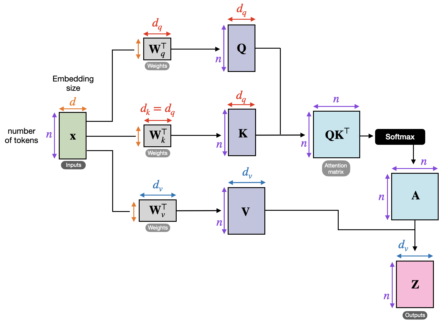
Self-attention calculations (image from https://sebastianraschka.com/blog/2023/self-attention-from-scratch.html)
class MultiHeadSelfAttention(nn.Module):
    def __init__(self, d, H):
        ''' Multi-Head Self-Attention module.
        Args:
            d: Embedding dimension.
            H: Number of attention heads.
        '''
        super(MultiHeadSelfAttention, self).__init__()
        assert d % H == 0, "Embedding dimension must be divisible by number of heads."
        self.d = d
        self.H = H
        self.d_k = d // H  # Dimension per head

        self.qkv = nn.Linear(d, 3*d)  # Combined query, key, value projection
        self.out = nn.Linear(d, d)  # Output projection

    def forward(self, X):
        '''
        Forward pass through the Multi-Head Self-Attention module.
        Args:
            X: Input tensor of shape (B, T, d).
        Returns:
            Output tensor of shape (B, T, d).
        '''
        B, T, d = X.shape
        assert d == self.d, f'Input embedding dimension {d} does not match model dimension {self.d}.'

        # Linear projections
        qkv = self.qkv(X)
        q,k,v = qkv.chunk(3, dim=-1)  # Each is (B, T, d) ---> form queries, keys, values

        # split into heads
        q_reshaped = q.view(B, T, self.H, self.d_k).transpose(1,2)  # (B, H, T, d_k)
        k_reshaped = k.view(B, T, self.H, self.d_k).transpose(1,2)  # (B, H, T, d_k)
        v_reshaped = v.view(B, T, self.H, self.d_k).transpose(1,2)  # (B, H, T, d_k)

        # Scaled dot-product attention
        k_transpose = k_reshaped.transpose(-2, -1)  # (B, H, d_k, T)
        QK = q_reshaped @ k_transpose # (B, H, T, T) ---> QK[b,h,i] stores the similarity of token i to all tokens in the sequence
        attn = QK.softmax(dim=-1) # (B, H, T, T) ---> attn[b,h,i] stores how much token i attends to all tokens in the sequence

        # alternative computation of softmax
        # alt_computation = QK.exp() / QK.exp().sum(dim=-1, keepdim=True)
        # assert torch.allclose(attn, alt_computation, atol=1e-5)

        # output calculation
        out = attn @ v_reshaped  # (B, H, T, d_k)
        out = out.transpose(1,2).contiguous().view(B, T, d) # (B, T, d) ---> put together all the heads
        out = self.out(out)
        return out
3. Training
3.1. Preparing the dataset
class DeEnPairs(Dataset):
    def __init__(self, dataset):
        self.de = dataset["de"]
        self.en = dataset["en"]

    def __len__(self):
        return len(self.de)

    def __getitem__(self, i):
        return self.de[i], self.en[i]

def make_causal_collate(tok, block_size=256, train_on_source=False):

    PAD_id = tok.pad_token_id
    BOS_id = tok.bos_token_id
    EOS_id = tok.eos_token_id

    def encode_plain(text):
        # Raw subword IDs, no BOS/EOS added automatically
        return tok(text, add_special_tokens=False)["input_ids"]

    def collate(batch):
        input_ids_list, labels_list, attn_list, end_of_DE_list = [], [], [], []

        for de_txt, en_txt in batch:
            de_ids = encode_plain(de_txt)
            en_ids = encode_plain(en_txt)

            # Build: [de, BOS, en, EOS]
            seq = de_ids + [BOS_id] + en_ids + [EOS_id]

            x = torch.tensor(seq, dtype=torch.long)

            # mask source part (German + the BOS boundary) unless you also want LM on DE
            # find BOS position we inserted as English boundary
            bos_pos = (x == BOS_id).nonzero(as_tuple=True)[0][0].item()

            # Labels = next-token targets. we shift inputs by one implicitly via CE on logits[:, :-1] vs labels[:, 1:]
            y = x.clone()[1:]

            if not train_on_source:
                y[:bos_pos] = -100  # ignore German and the BOS token

            # last token has no next-token label; safe to keep (HF shifts internally),
            # but many people prefer to mask last position explicitly:
            # y[-1] = -100

            attn = torch.ones_like(x, dtype=torch.long)  # 1 for real tokens; padding will be 0

            input_ids_list.append(x)
            labels_list.append(y)
            attn_list.append(attn)
            end_of_DE_list.append(bos_pos+1)

        # Pad to batch max length
        input_ids = pad_sequence(input_ids_list, batch_first=True, padding_value=PAD_id)
        labels    = pad_sequence(labels_list,    batch_first=True, padding_value=-100)
        attention = pad_sequence(attn_list,      batch_first=True, padding_value=0)
        end_of_DE_list = torch.tensor(end_of_DE_list, dtype=torch.long)

        # If sequence still exceeds block_size after padding logic (rare), hard cut at right edge:
        if input_ids.size(1) > block_size:
            input_ids = input_ids[:, -block_size:]
            labels    = labels[:,    -block_size:]
            attention = attention[:, -block_size:]

        return {"input_ids": input_ids, "attention_mask": attention, "labels": labels, "end_of_DE": end_of_DE_list}

    return collate

train_ds = DeEnPairs(ds_train)
valid_ds = DeEnPairs(ds_valid)

collate = make_causal_collate(tok, block_size=256, train_on_source=True)
train_dl = DataLoader(train_ds, batch_size=64, shuffle=True, collate_fn=collate)
batch = next(iter(train_dl))

# 1 if there is a real token, 0 if padding
print('Attention masks:\n',batch['attention_mask'][0],'\n')

# indices of tokens in the vocabulary. remember 58101 is <bos>, 0 is <eos>, 58100 is <pad>
print('Input ids:\n',batch['input_ids'][0],'\n')

# the beginning idx of the English part (after German + <bos>)
print('End of German sentences:\n',batch['end_of_DE'][0],'\n')

# the idx of the next token to predict, -100 if ignored (German + <bos> + padding)
print('Labels:\n',batch['labels'][0],'\n')

# print the actual text
for i in range(batch['attention_mask'][0].sum()):
    print(batch['input_ids'][0][i].item(), tok.decode(batch['input_ids'][0][i].item()), sep='\t')
Attention masks:
 tensor([1, 1, 1, 1, 1, 1, 1, 1, 1, 1, 1, 1, 1, 1, 1, 1, 1, 1, 1, 1, 1, 1, 1, 1,
        1, 1, 1, 1, 1, 1, 1, 1, 1, 1, 1, 1, 1, 1, 1, 1, 1, 1, 1, 1, 1, 1, 1, 1,
        1, 1, 1, 0, 0, 0, 0, 0, 0, 0, 0, 0, 0, 0, 0, 0, 0, 0, 0, 0, 0, 0, 0, 0,
        0, 0, 0])

Input ids:
 tensor([  525, 17593,   222, 41377,    15, 19943, 16778,    37,    94, 16167,
            2,   145,  2229, 12317,  4691, 22799,     3, 58101,    93,    17,
         7565,    18,     7,    39,    17,  6409,    15,  1730,   175,    17,
            6,  9401,    32,    14,    17, 12662,     5,    17,  9691,     7,
           88,  1032,    17, 19376,    17, 27499,    17, 16391,     6,     3,
            0, 58100, 58100, 58100, 58100, 58100, 58100, 58100, 58100, 58100,
        58100, 58100, 58100, 58100, 58100, 58100, 58100, 58100, 58100, 58100,
        58100, 58100, 58100, 58100, 58100])

End of German sentences:
 tensor(18)

Labels:
 tensor([17593,   222, 41377,    15, 19943, 16778,    37,    94, 16167,     2,
          145,  2229, 12317,  4691, 22799,     3, 58101,    93,    17,  7565,
           18,     7,    39,    17,  6409,    15,  1730,   175,    17,     6,
         9401,    32,    14,    17, 12662,     5,    17,  9691,     7,    88,
         1032,    17, 19376,    17, 27499,    17, 16391,     6,     3,     0,
         -100,  -100,  -100,  -100,  -100,  -100,  -100,  -100,  -100,  -100,
         -100,  -100,  -100,  -100,  -100,  -100,  -100,  -100,  -100,  -100,
         -100,  -100,  -100,  -100])

525	Eine
17593	Figur
222	eines
41377	orientalisch
15	en
19943	Mannes
16778	sitzt
37	auf
94	einer
16167	Mauer
2	,
145	vor
2229	einigen
12317	weißen
4691	Wohn
22799	häusern
3	.
58101	<bos>
93	A
17
7565	figur
18	e
7	of
39	an
17
6409	ori
15	en
1730	tal
175	man
17
6	s
9401	its
32	on
14	a
17
12662	wall
5	in
17
9691	front
7	of
88	so
1032	me
17
19376	white
17
27499	apartment
17
16391	building
6	s
3	.
0	</s>
3.2. Our training pipeline
In practice, we train these models efficiently by predicting many next tokens in parallel. Suppose our target sequence has length D. Instead of creating D separate training examples (each with a different context), we process the whole sequence at once. We feed the model the input [x₁, x₂, …, x_{D-1}], and we ask it to predict [x₂, x₃, …, x_D]. In other words, for every position, the model tries to guess “what comes next.” This produces D-1 predictions from a single forward pass. During inference, the model still generates one token at a time, but during training we can supervise all positions simultaneously, which makes learning much faster. The important distinction is: training = parallel next-token prediction across the sequence, generation = sequential prediction, one token at a time.
So now, we implement a causal attention mechanism that predicts token $i$ conditioned to all tokens until $i$.
class MultiHeadCausalSelfAttention(nn.Module):
    def __init__(self, d, H):
        ''' Multi-Head Self-Attention module.
        Args:
            d: Embedding dimension.
            H: Number of attention heads.
        '''
        super(MultiHeadCausalSelfAttention, self).__init__()
        assert d % H == 0, "Embedding dimension must be divisible by number of heads."
        self.d = d
        self.H = H
        self.d_k = d // H  # Dimension per head

        self.qkv = nn.Linear(d, 3*d)  # Combined query, key, value projection
        self.out = nn.Linear(d, d)  # Output projection

    def forward(self, X):
        '''
        Forward pass through the Multi-Head Self-Attention module.
        Args:
            X: Input tensor of shape (B, T, d).
            eng_start_idx: Tensor of shape (B,) indicating the start index of the English part in each sequence.
        Returns:
            Output tensor of shape (B, T, d).
        '''
        B, T, d = X.shape
        assert d == self.d, f'Input embedding dimension {d} does not match model dimension {self.d}.'

        # Linear projections
        qkv = self.qkv(X)
        q,k,v = qkv.chunk(3, dim=-1)  # Each is (B, T, d) ---> form queries, keys, values

        # split into heads
        q_reshaped = q.view(B, T, self.H, self.d_k).transpose(1,2)  # (B, H, T, d_k)
        k_reshaped = k.view(B, T, self.H, self.d_k).transpose(1,2)  # (B, H, T, d_k)
        v_reshaped = v.view(B, T, self.H, self.d_k).transpose(1,2)  # (B, H, T, d_k)

        # Scaled dot-product attention
        k_transpose = k_reshaped.transpose(-2, -1)  # (B, H, d_k, T)
        QK = q_reshaped @ k_transpose # (B, H, T, T) ---> QK[b,h,i] stores the similarity of token i to all tokens in the sequence

        # create the causal mask
        causal_mask = torch.tril(torch.ones((T, T), device=X.device)).unsqueeze(0).unsqueeze(0)  # (1, 1, T, T)
        QK = QK.masked_fill(causal_mask == 0, float('-inf'))
        attn = QK.softmax(dim=-1) # (B, H, T, T) ---> attn[b,h,i] stores how much token i attends to all tokens in the sequence

        # output calculation
        out = attn @ v_reshaped  # (B, H, T, d_k)
        out = out.transpose(1,2).contiguous().view(B, T, d) # (B, T, d) ---> put together all the heads
        out = self.out(out)
        return out
3.3. Build the network
T = 256         # Context length (sequence length)
V = len(tok)    # Vocabulary size (for embeddings)
N = 12          # Number of Transformer blocks
d = 256         # Embedding dimension
H = 8           # Number of attention heads

input_emb = create_embedding(V, d) # Input embedding
pos_emb   = create_embedding(T, d) # Positional embedding

mhsa = MultiHeadCausalSelfAttention(d, H)
transf_block = Block(mhsa, d, 4*d, dropout=0.1)
norm_layer = nn.LayerNorm(d)
output_layer = nn.Linear(d, V)  # Output layer to project to vocabulary size

model = TransformerNetwork(
    T=T, # max seq length
    N=N, # num transformer blocks
    input_emb=input_emb, # Input embedding layer/module.
    pos_emb=pos_emb, # Positional embedding layer/module.
    transf_block=transf_block, # A single Transformer block (to be repeated N times).
    norm_layer=norm_layer, # Normalization layer/module (e.g., LayerNorm).
    output_layer=output_layer # Output layer/module (e.g., to map to data space).
)

print(model)
print('Number of parameters in the model:', sum(p.numel() for p in model.parameters()) )

optimizer = torch.optim.AdamW(model.parameters(), lr=5e-4, weight_decay=1e-3, betas=(0.9, 0.99), eps=1e-8)

model = model.to(device)

# state = torch.load('transformer_deen_T256_N12_d256_H8_can_generate_german.pth', map_location=device)
# model.load_state_dict(state)
TransformerNetwork(
  (input_emb): Embedding(58102, 256)
  (pos_emb): Embedding(256, 256)
  (transf_blocks): ModuleList(
    (0-11): 12 x Block(
      (mhsa): MultiHeadCausalSelfAttention(
        (qkv): Linear(in_features=256, out_features=768, bias=True)
        (out): Linear(in_features=256, out_features=256, bias=True)
      )
      (ffn): Sequential(
        (0): Linear(in_features=256, out_features=1024, bias=True)
        (1): ReLU()
        (2): Linear(in_features=1024, out_features=256, bias=True)
      )
      (norm1): LayerNorm((256,), eps=1e-05, elementwise_affine=True)
      (norm2): LayerNorm((256,), eps=1e-05, elementwise_affine=True)
      (dropout): Dropout(p=0.1, inplace=False)
    )
  )
  (norm_layer): LayerNorm((256,), eps=1e-05, elementwise_affine=True)
  (output_layer): Linear(in_features=256, out_features=58102, bias=True)
)
Number of parameters in the model: 30662134
/tmp/ipykernel_616401/352975203.py:33: FutureWarning: You are using `torch.load` with `weights_only=False` (the current default value), which uses the default pickle module implicitly. It is possible to construct malicious pickle data which will execute arbitrary code during unpickling (See https://github.com/pytorch/pytorch/blob/main/SECURITY.md#untrusted-models for more details). In a future release, the default value for `weights_only` will be flipped to `True`. This limits the functions that could be executed during unpickling. Arbitrary objects will no longer be allowed to be loaded via this mode unless they are explicitly allowlisted by the user via `torch.serialization.add_safe_globals`. We recommend you start setting `weights_only=True` for any use case where you don't have full control of the loaded file. Please open an issue on GitHub for any issues related to this experimental feature.
  state = torch.load('transformer_deen_T256_N12_d256_H8_can_generate_german.pth', map_location=device)
---------------------------------------------------------------------------
NameError                                 Traceback (most recent call last)
Cell In[9], line 35
     33 state = torch.load('transformer_deen_T256_N12_d256_H8_can_generate_german.pth', map_location=device)
     34 model.load_state_dict(state)
---> 35 print(aaa)

NameError: name 'aaa' is not defined
3.4. Train the network
# train the network
for epoch in range(20):
    model.train()
    total_loss = 0.0
    for i,batch in enumerate(train_dl):
        input_ids = batch['input_ids'].to(device)
        labels = batch['labels'].to(device)
        eng_start_idx = batch['end_of_DE'].to(device)

        optimizer.zero_grad()
        outputs = model(input_ids)  # (B, T, V)
        logits = outputs[:, :-1, :].contiguous()  # (B, T-1, V)

        loss = F.cross_entropy(logits.view(-1, V), labels.view(-1), ignore_index=-100)
        loss.backward()
        optimizer.step()

        total_loss += loss.item()

        if i % 100 == 0:
            print(f'Processing batch {i}/{len(train_dl)}. Mean loss so far: {total_loss/(i+1):.4f}')

    avg_loss = total_loss / len(train_dl)
    print(f'Epoch {epoch+1}, Training Loss: {avg_loss:.4f}')

torch.save(model.state_dict(), 'transformer_deen.pth')
Processing batch 0/454. Mean loss so far: 11.1316
Processing batch 100/454. Mean loss so far: 6.0472
Processing batch 200/454. Mean loss so far: 5.1690
Processing batch 300/454. Mean loss so far: 4.7178
Processing batch 400/454. Mean loss so far: 4.4251
Epoch 1, Training Loss: 4.3016
Processing batch 0/454. Mean loss so far: 3.5583
Processing batch 100/454. Mean loss so far: 3.2004
Processing batch 200/454. Mean loss so far: 3.1463
Processing batch 300/454. Mean loss so far: 3.1020
Processing batch 400/454. Mean loss so far: 3.0596
Epoch 2, Training Loss: 3.0323
Processing batch 0/454. Mean loss so far: 2.8784
Processing batch 100/454. Mean loss so far: 2.7206
Processing batch 200/454. Mean loss so far: 2.6985
Processing batch 300/454. Mean loss so far: 2.6770
Processing batch 400/454. Mean loss so far: 2.6592
Epoch 3, Training Loss: 2.6491
Processing batch 0/454. Mean loss so far: 2.4186
Processing batch 100/454. Mean loss so far: 2.4207
Processing batch 200/454. Mean loss so far: 2.4191
Processing batch 300/454. Mean loss so far: 2.4177
Processing batch 400/454. Mean loss so far: 2.4111
Epoch 4, Training Loss: 2.4055
Processing batch 0/454. Mean loss so far: 2.1825
Processing batch 100/454. Mean loss so far: 2.2375
Processing batch 200/454. Mean loss so far: 2.2403
Processing batch 300/454. Mean loss so far: 2.2430
Processing batch 400/454. Mean loss so far: 2.2384
Epoch 5, Training Loss: 2.2337
Processing batch 0/454. Mean loss so far: 2.2638
Processing batch 100/454. Mean loss so far: 2.0781
Processing batch 200/454. Mean loss so far: 2.0903
Processing batch 300/454. Mean loss so far: 2.0961
Processing batch 400/454. Mean loss so far: 2.1039
Epoch 6, Training Loss: 2.1036
Processing batch 0/454. Mean loss so far: 2.0014
Processing batch 100/454. Mean loss so far: 1.9786
Processing batch 200/454. Mean loss so far: 1.9838
Processing batch 300/454. Mean loss so far: 1.9911
Processing batch 400/454. Mean loss so far: 1.9965
Epoch 7, Training Loss: 1.9970
Processing batch 0/454. Mean loss so far: 1.9444
Processing batch 100/454. Mean loss so far: 1.8606
Processing batch 200/454. Mean loss so far: 1.8752
Processing batch 300/454. Mean loss so far: 1.8913
Processing batch 400/454. Mean loss so far: 1.8993
Epoch 8, Training Loss: 1.9066
Processing batch 0/454. Mean loss so far: 1.6859
Processing batch 100/454. Mean loss so far: 1.7814
Processing batch 200/454. Mean loss so far: 1.7992
Processing batch 300/454. Mean loss so far: 1.8133
Processing batch 400/454. Mean loss so far: 1.8245
Epoch 9, Training Loss: 1.8286
Processing batch 0/454. Mean loss so far: 1.7428
Processing batch 100/454. Mean loss so far: 1.7061
Processing batch 200/454. Mean loss so far: 1.7296
Processing batch 300/454. Mean loss so far: 1.7408
Processing batch 400/454. Mean loss so far: 1.7550
Epoch 10, Training Loss: 1.7606
Processing batch 0/454. Mean loss so far: 1.6196
Processing batch 100/454. Mean loss so far: 1.6392
Processing batch 200/454. Mean loss so far: 1.6609
Processing batch 300/454. Mean loss so far: 1.6790
Processing batch 400/454. Mean loss so far: 1.6942
Epoch 11, Training Loss: 1.7006
Processing batch 0/454. Mean loss so far: 1.5412
Processing batch 100/454. Mean loss so far: 1.5813
Processing batch 200/454. Mean loss so far: 1.6037
Processing batch 300/454. Mean loss so far: 1.6211
Processing batch 400/454. Mean loss so far: 1.6373
Epoch 12, Training Loss: 1.6448
Processing batch 0/454. Mean loss so far: 1.5117
Processing batch 100/454. Mean loss so far: 1.5385
Processing batch 200/454. Mean loss so far: 1.5619
Processing batch 300/454. Mean loss so far: 1.5775
Processing batch 400/454. Mean loss so far: 1.5889
Epoch 13, Training Loss: 1.5935
Processing batch 0/454. Mean loss so far: 1.3743
Processing batch 100/454. Mean loss so far: 1.4866
Processing batch 200/454. Mean loss so far: 1.5096
Processing batch 300/454. Mean loss so far: 1.5286
Processing batch 400/454. Mean loss so far: 1.5441
Epoch 14, Training Loss: 1.5500
Processing batch 0/454. Mean loss so far: 1.4222
Processing batch 100/454. Mean loss so far: 1.4365
Processing batch 200/454. Mean loss so far: 1.4626
Processing batch 300/454. Mean loss so far: 1.4873
Processing batch 400/454. Mean loss so far: 1.5038
Epoch 15, Training Loss: 1.5086
Processing batch 0/454. Mean loss so far: 1.3181
Processing batch 100/454. Mean loss so far: 1.4103
Processing batch 200/454. Mean loss so far: 1.4276
Processing batch 300/454. Mean loss so far: 1.4486
Processing batch 400/454. Mean loss so far: 1.4640
Epoch 16, Training Loss: 1.4719
Processing batch 0/454. Mean loss so far: 1.3642
Processing batch 100/454. Mean loss so far: 1.3767
Processing batch 200/454. Mean loss so far: 1.3968
Processing batch 300/454. Mean loss so far: 1.4167
Processing batch 400/454. Mean loss so far: 1.4323
Epoch 17, Training Loss: 1.4374
Processing batch 0/454. Mean loss so far: 1.3088
Processing batch 100/454. Mean loss so far: 1.3422
Processing batch 200/454. Mean loss so far: 1.3636
Processing batch 300/454. Mean loss so far: 1.3824
Processing batch 400/454. Mean loss so far: 1.3981
Epoch 18, Training Loss: 1.4056
Processing batch 0/454. Mean loss so far: 1.2703
Processing batch 100/454. Mean loss so far: 1.3162
Processing batch 200/454. Mean loss so far: 1.3311
Processing batch 300/454. Mean loss so far: 1.3505
Processing batch 400/454. Mean loss so far: 1.3692
Epoch 19, Training Loss: 1.3765
Processing batch 0/454. Mean loss so far: 1.2532
Processing batch 100/454. Mean loss so far: 1.2835
Processing batch 200/454. Mean loss so far: 1.3037
Processing batch 300/454. Mean loss so far: 1.3248
Processing batch 400/454. Mean loss so far: 1.3416
Epoch 20, Training Loss: 1.3480
3.5. Example model outputs
Finally, we take a test input and let model translate it. We give the German sentences as input and let model predict the next tokens.
@torch.no_grad()
def generate(model, idx, max_new_tokens, temperature=1.0, do_sample=False, top_k=None):
    """
        Parameters:
        -----------
        model: The trained Transformer model.
        idx: Tensor of shape (B, T) containing the initial sequence of token indices.
        max_new_tokens: Number of new tokens to generate.
        temperature: Controls the randomness of predictions by scaling the logits.
        do_sample: If True, sample from the probability distribution; if False, take the most likely token.
        top_k: If specified, restricts sampling to the top_k most probable tokens
    """
    for _ in range(max_new_tokens):
        # forward the model to get the logits for the index in the sequence
        logits = model(idx)
        # pluck the logits at the final step and scale by desired temperature
        logits = logits[:, -1, :] / temperature
        # optionally crop the logits to only the top k options
        if top_k is not None:
            v, _ = torch.topk(logits, top_k)
            logits[logits < v[:, [-1]]] = -float('Inf')
        # apply softmax to convert logits to (normalized) probabilities
        probs = F.softmax(logits, dim=-1)
        # either sample from the distribution or take the most likely element
        if do_sample:
            idx_next = torch.multinomial(probs, num_samples=1)
        else:
            _, idx_next = torch.topk(probs, k=1, dim=-1)
        # append sampled index to the running sequence and continue
        idx = torch.cat((idx, idx_next), dim=1)

    return idx

# generate starting from a test sentence
valid_dl = DataLoader(valid_ds, batch_size=64, shuffle=True, collate_fn=collate)
batch = next(iter(valid_dl))

i = 0
input_ids, attention_mask, end_of_de = batch['input_ids'][i:i+1], batch['attention_mask'][i:i+1], batch['end_of_DE'][i:i+1]
input_ids, attention_mask, end_of_de = input_ids.to(device), attention_mask.to(device), end_of_de.to(device)

# translate
print('Input:\t\t', tok.decode(input_ids[0,:end_of_de]))
print('Output:\t\t', tok.decode(input_ids[0][end_of_de:]))
model_output = generate(model, input_ids[:,:end_of_de], 50, temperature=1.0, do_sample=False, top_k=None)
print('Generated:\t', tok.decode(model_output[0][end_of_de:]))

# generate German sentence
# print('Input:\t\t', tok.decode(input_ids[0,:end_of_de//2]))
# print('Output:\t\t', tok.decode(input_ids[0][end_of_de//2:]))
# model_output = generate(model, input_ids[:,:end_of_de//2], 50, temperature=1.0, do_sample=False, top_k=None)
# print('Generated:\t', tok.decode(model_output[0][end_of_de//2:]))
Input:		 Zwei Männer sind an einem hellen, sonnigen Tag unterwegs, um ein paar Fische im See zu fangen.<bos>
Output:		 Two men are out on a bright, sunny day attempting to catch some fish on the lake.</s> <pad> <pad> <pad> <pad> <pad> <pad> <pad> <pad> <pad> <pad> <pad> <pad> <pad> <pad>
Generated:	 Two men are enjoying a bright pond down a sideway toy in lake a lake.</s> e store's lake.</s> e store.</s> es.</s> es
4. Vision transformers
Vision Transformers (ViTs) bring the transformer architecture—originally designed for natural language processing—into computer vision. Instead of processing images with convolutional filters, a ViT splits an image into fixed-size patches (for example, 16×16 pixels), flattens them, and linearly projects each patch into an embedding vector. These embeddings form a sequence, much like a sentence in NLP, and are fed into a transformer encoder. A special “class token” is prepended to the sequence and its final hidden state serves as the representation for the whole image, which can then be used for classification or downstream tasks. Positional encodings are also added, since transformers themselves have no inherent sense of order or spatial arrangement.
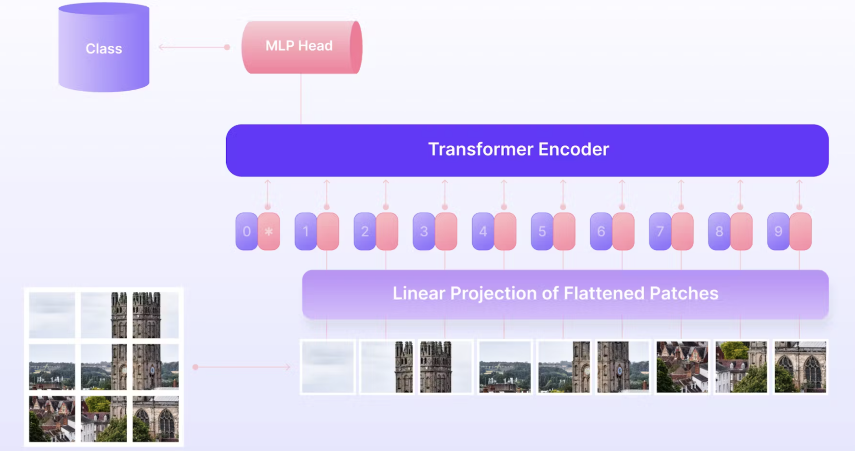
A demonstration of vision transformers (image from https://encord.com/blog/vision-transformers/)
What makes ViTs powerful is their ability to model long-range dependencies: any patch can attend to any other patch, allowing the network to capture global structure in an image. Unlike convolutional networks, which focus on local receptive fields and build hierarchical features layer by layer, ViTs start with a global receptive field from the very first layer. This flexibility comes at the cost of needing large amounts of data (or pretraining on large datasets like ImageNet-21k) and careful regularization. Once pretrained, ViTs transfer very well across tasks, and they’ve become state-of-the-art not just in classification, but also in detection, segmentation, and even generative vision models.
4.1. ViT implementation
The main difference to previous implementation is the addition of the CLS token.
class VisionTransformer(nn.Module):
    def __init__(self, T, N, input_emb, pos_emb, transf_block, norm_layer, output_layer):
        ''' Transformer network with N blocks, context length T, and given components.
        Args:
            T: Context length (sequence length).
            N: Number of Transformer blocks.
            input_emb: Input embedding layer/module.
            pos_emb: Positional embedding layer/module.
            transf_block: A single Transformer block (to be repeated N times).
            norm_layer: Normalization layer/module (e.g., LayerNorm).
            output_layer: Output layer/module (e.g., for classification or regression).
        '''
        super(VisionTransformer, self).__init__()
        self.T = T
        self.input_emb = input_emb
        self.pos_emb = pos_emb
        self.transf_blocks = nn.ModuleList([transf_block for _ in range(N)])
        self.norm_layer = norm_layer
        self.output_layer = output_layer
        embed_dim = pos_emb.embedding_dim
        self.cls_token = nn.Parameter(torch.randn(1,1,embed_dim))

    @property
    def device(self):
        return next(self.parameters()).device

    @property
    def dtype(self):
        return next(self.parameters()).dtype

    @property
    def num_layers(self):
        return len(self.transf_blocks)

    @property
    def d(self):
        return self.input_emb.embedding_dim

    def forward(self, X):
        '''
        Forward pass through the Transformer network.
        Args:
            X: Input tensor of shape (batch_size, seq_length, input_dim), or (B,T,d).
        Returns:
            Output tensor after passing through the Transformer network - [B,output_dim].
        '''
        device = X.device
        B,T = X.shape[0:2]

        # Input embedding
        X  = self.input_emb(X)  # B,T,d

        # add CLS token
        cls_tokens = self.cls_token.repeat(B,1,1)
        X = torch.cat((cls_tokens, X), dim=1)
        T = T+1

        # positional embeddings
        P  = self.pos_emb(torch.arange(T, device=device)) # T,d
        P  = P.unsqueeze(0).expand(B, T, -1)  # B,T,d

        # adding positional embeddings
        X = X + P  # B,T,d

        # passing through Transformer blocks
        for block in self.transf_blocks:
            X = block(X)  # B,T,d

        class_token_final = X[:,0,:]

        # final normalization
        class_token_final = self.norm_layer(class_token_final)  # B,d

        # output layer
        out = self.output_layer(class_token_final)  # B,output_dim (depends on output_layer)

        return out
4.2. Build the network
This time,
- the embedding layers are simple MLPs.
- input length depends on the image and patch size.
patch_size = 8
T = int((32/patch_size)**2)     # Context length (sequence length)
N = 12      # Number of Transformer blocks
d = 256     # Embedding dimension
H = 16       # Number of attention heads
num_classes = 10 # number of output classes (for CIFAR-10)

input_emb = nn.Linear(3*(patch_size**2), d) # Input embedding
pos_emb   = nn.Embedding(T+1, d) # create_embedding(T+1, d) # Positional embedding

mhsa = MultiHeadSelfAttention(d, H)
transf_block = Block(mhsa, d, 4*d, dropout=0.1)
norm_layer = nn.LayerNorm(d)
output_layer = nn.Linear(d, num_classes)  # Output layer to project to vocabulary size

model = VisionTransformer(
    T=T, # max seq length
    N=N, # num transformer blocks
    input_emb=input_emb, # Input embedding layer/module.
    pos_emb=pos_emb, # Positional embedding layer/module.
    transf_block=transf_block, # A single Transformer block (to be repeated N times).
    norm_layer=norm_layer, # Normalization layer/module (e.g., LayerNorm).
    output_layer=output_layer # Output layer/module (e.g., to map to data space).
)

print(model)
print('Number of parameters in the model:', sum(p.numel() for p in model.parameters()) )

optimizer = torch.optim.AdamW(model.parameters(), lr=1e-3, weight_decay=1e-3, betas=(0.9, 0.99), eps=1e-8)
model = model.to(device)
VisionTransformer(
  (input_emb): Linear(in_features=192, out_features=256, bias=True)
  (pos_emb): Embedding(17, 256)
  (transf_blocks): ModuleList(
    (0-11): 12 x Block(
      (mhsa): MultiHeadSelfAttention(
        (qkv): Linear(in_features=256, out_features=768, bias=True)
        (out): Linear(in_features=256, out_features=256, bias=True)
      )
      (ffn): Sequential(
        (0): Linear(in_features=256, out_features=1024, bias=True)
        (1): ReLU()
        (2): Linear(in_features=1024, out_features=256, bias=True)
      )
      (norm1): LayerNorm((256,), eps=1e-05, elementwise_affine=True)
      (norm2): LayerNorm((256,), eps=1e-05, elementwise_affine=True)
      (dropout): Dropout(p=0.1, inplace=False)
    )
  )
  (norm_layer): LayerNorm((256,), eps=1e-05, elementwise_affine=True)
  (output_layer): Linear(in_features=256, out_features=10, bias=True)
)
Number of parameters in the model: 846858
4.3. Training functions
We train the model on CIFAR10 dataset.
test_transform = transforms.Compose([transforms.ToTensor(),
                                     transforms.Normalize([0.49139968, 0.48215841, 0.44653091], [0.24703223, 0.24348513, 0.26158784])
                                     ])
# For training, we add some augmentation. Networks are too powerful and would overfit.
train_transform = transforms.Compose([transforms.RandomHorizontalFlip(),
                                      transforms.RandomResizedCrop((32,32),scale=(0.8,1.0),ratio=(0.9,1.1)),
                                      transforms.ToTensor(),
                                      transforms.Normalize([0.49139968, 0.48215841, 0.44653091], [0.24703223, 0.24348513, 0.26158784])
                                     ])

# Loading the training dataset. We need to split it into a training and validation part
# We need to do a little trick because the validation set should not use the augmentation.
train_dataset = CIFAR10(root='data/', train=True, transform=train_transform, download=True)
val_dataset   = CIFAR10(root='data/', train=True, transform=test_transform,  download=True)

train_dl = DataLoader(train_dataset, batch_size=128, shuffle=True, num_workers=2, pin_memory=True)
val_dl   = DataLoader(val_dataset, batch_size=256, shuffle=False, num_workers=2, pin_memory=True)

def img_to_patch(x, patch_size):
    """
    Inputs:
        x - torch.Tensor representing the image of shape [B, C, H, W]
        patch_size - Number of pixels per dimension of the patches (integer)
    """
    B, C, H, W = x.shape
    x = x.reshape(B, C, H//patch_size, patch_size, W//patch_size, patch_size)
    x = x.permute(0, 2, 4, 1, 3, 5) # [B, H', W', C, p_H, p_W]
    x = x.flatten(1,2)              # [B, H'*W', C, p_H, p_W]
    x = x.flatten(2,4)          # [B, H'*W', C*p_H*p_W]
    return x

# X = img_to_patch(X, self.patch_size)  # B,T,d
Files already downloaded and verified
Files already downloaded and verified
4.4. Training loop
# train the network
for epoch in range(20):
    model.train()
    total_accuracy = 0.0
    for i,batch in enumerate(train_dl):
        X, y = batch
        X, y = X.to(device), y.to(device)

        X = img_to_patch(X, patch_size)
        optimizer.zero_grad()
        logits = model(X)  # (B, num_classes)
        loss = F.cross_entropy(logits, y)
        accuracy = (logits.argmax(dim=-1) == y).float().mean()
        loss.backward()
        optimizer.step()
        total_accuracy += accuracy.item()
        if i % 100 == 0:
            print(f'Processing batch {i}/{len(train_dl)}. Mean accuracy so far: {total_accuracy/(i+1):.4f}')

    # now validate
    model.eval()
    total_val_accuracy = 0.0
    with torch.no_grad():
        for i,batch in enumerate(val_dl):
            X, y = batch
            X, y = X.to(device), y.to(device)

            X = img_to_patch(X, patch_size)
            logits = model(X)  # (B, num_classes)
            accuracy = (logits.argmax(dim=-1) == y).float().mean()
            total_val_accuracy += accuracy.item()
        print(f'Epoch {epoch+1}, Training Accuracy: {total_accuracy/len(train_dl):.4f}, Validation Accuracy: {total_val_accuracy/len(val_dl):.4f}')